How the difference is computed

This page describes what Compute difference actually computes: the method, the settings it uses, and how the numbers in the panel follow from its output. It is here so you can judge whether a result is trustworthy and explain it to someone who asks.

The method in one sentence

Both revisions are rasterized into 2.5D elevation grids on an identical pixel grid, revision A’s grid is subtracted from revision B’s, and the result is masked to your boundary and stored as a GeoTIFF that everything else reads.

2.5D, not 3D

A 2.5D grid holds one height per cell - the smoothed height of the survey points that fell in it. It is the right model for a seabed and the wrong model for anything vertical. Overhangs, the sides of a pipe, the walls of a structure, the underside of a mattress: none of these are surfaces the grid can represent, so change on them is not measured. The panel repeats this caveat in Method & calculation settings for exactly this reason.

The Pipeline

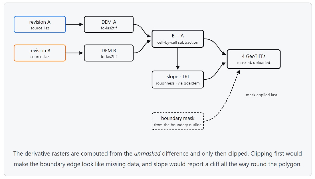
Step by step

Load and validate. - The job loads the account, project and sub-project, then checks that both revisions exist, are processingState: 200, and have a preserved source file. A missing boundary or a missing source file fails the run with a specific message.
Download both sources. - Each revision’s preserved .laz is fetched via its signed URL into the job’s working directory.
Measure the surveys. - Each survey’s horizontal extent is read from its file.
Choose the grid. - The area actually gridded is your boundary’s extent intersected with the area both surveys cover, snapped outward to whole cells. That intersection is what stops a huge boundary from producing a huge, mostly empty raster. A boundary that does not overlap the data at all fails here, with a message saying so.
Turn each survey into a grid. - One elevation grid per survey, on that exact same grid, so the two are cell-for-cell aligned - without that alignment a subtraction would compare offset cells and invent change that is not there. The boundary is applied here too, so points far outside it are never processed.

Each cell’s height is a Gaussian-weighted mean of the points near it: points closer to the cell center count for more, with the weighting controlled by sigma and the neighborhood by radius. Cells with no points in reach are left as NoData.
Subtract. B − A. - Cell by cell. A cell has no answer if either survey had no answer there - that is exactly what “observable in both revisions” means, and where the transparent patches on the map come from.
Derive the three companion rasters - From the unmasked difference:

Raster	Method	Reads as
Slope	Horn’s slope algorithm	Degrees. The steepness of the change surface, not of the seabed.
Ruggedness	Wilson’s Terrain Ruggedness Index	How much the change varies within a cell’s neighborhood.
Roughness	Largest difference to any neighboring cell	Isolated spikes, often data artefacts.

All three are standard GDAL terrain measures (gdaldem), so the definitions are public and the numbers are reproducible outside FieldTwin.

Clip to the boundary. - The boundary outline - including any holes - is turned into a mask on the same grid and applied to the difference and all three derived rasters. Everything outside becomes “no answer”.
Store the four rasters with the result - Store it along with the settings that produced them. This is what makes a comparison reappear instantly instead of recomputing, and what the GeoTIFF button hands you.
Build the surface you see. - The difference raster is converted into a drawable surface the same way a survey is, and attached to survey A’s point cloud so the 3D view can render it.

The job also backfills a missing elevation raster on either revision from the DEM it just built - which is why computing one difference can fix a profile that previously said the revision had no raster.

Parameters

These are the values Method & calculation settings shows on a finished result, and they are stored with it - so a comparison run last year is still interpretable even if the defaults have since changed.

Setting	Default	What it means
Method	Elevation difference of two 2.5D grids	One height per cell, subtracted.
Method version	1	Recorded so an old result stays comparable if the method changes.
Difference	B − A	Positive means B is higher than A.
How points become a height	Gaussian-weighted mean	Points nearer the cell center count for more.
Grid resolution	0.5 project units	The cell size.
Gaussian sigma	same as the resolution	The smoothing width. Larger is smoother.
Search radius	2σ, expressed in cells	How far from a cell center points are gathered.
Change threshold	none	No noise floor: every difference counts, including survey noise.

Resolution, sigma and radius are set per deployment rather than per comparison, so everyone in an environment gets comparable results. Whoever runs the deployment can change them; a user cannot.

Choosing a resolution is a trade-off

Finer cells resolve smaller features but need denser surveys: a cell with too few points in reach becomes NoData, so a finer grid usually lowers coverage. Coarser cells raise coverage and smooth detail away. The default 0.5 units suits typical seabed survey densities; these are per-deployment settings rather than per-run ones, so a change affects every new comparison.

How volumes are integrated

Volumes are not computed by the job. The panel asks the analysis service to integrate the stored difference raster inside the boundary, which is why the numbers appear a moment after the map and are recomputed when you move the boundary.

For each raster cell whose center falls inside the boundary’s outer ring and outside all of its holes:

The cell counts toward the analysis area - the total you drew.
Its value is classified. NoData, non-finite, or out-of-supported-range values are counted separately and contribute nothing further.
A usable value counts toward the observed area, and contributes value × cellArea to the net volume, and to either deposition (≥ 0) or erosion (< 0).

So:

Net change = Σ (cell difference × cell area) over observed cells
Deposition = the same sum restricted to positive cells
Erosion = the same sum restricted to negative cells
Coverage = observed area ÷ analysis area, falling back to the cell-count ratio

Because inclusion is decided by the cell center, a boundary edge is accurate to about half a cell. At the default resolution that is 0.25 units of edge uncertainty - irrelevant for a 50 m polygon, significant for a 2 m one.

The service also returns a decimated triangulated mesh of the changed volume - capped at a few thousand cells and Delaunay-triangulated from the cell centers - which is what Volume mesh displays. The mesh is a preview of the shape; the volume figures come from every observed cell at full resolution.

When the integration cannot answer

What the panel says	What it means
Boundary did not contain any valid raster values	Every cell inside the boundary is unanswerable - the boundary is off the data, or the two surveys do not overlap there.
Raster contained volume values outside the supported range	The map holds values the integration will not trust. Retrying re-reads it from storage rather than from cache.
A read failure	The stored raster could not be read at all, usually an expired link or a storage problem.

The distinction matters: the first is a question about your boundary, the second and third are about the data, and only the last is worth escalating.

Reproducibility

Two runs of the same pair with the same boundary and the same parameters produce the same raster, and the panel exploits that: selecting a pair and a boundary that already have a stored result reuses it rather than recomputing. The boundary hash is what makes “the same boundary” decidable - nudge the shape and you get a new comparison rather than a silently stale one.

Recompute exists for the case the hash cannot see: the inputs changed, not the geometry. Re-import a survey and recompute to pick it up.