Point Cloud Comparison
This will display the dialog for the Point Cloud Comparison Tool that allows you to as an example compare point clouds from inspections of an asset or pipeline and detect any changes over time. This can be usueful to detect the dangers of scouring for subsea assets or pipelines.
With this tool you can easily do the following:
Fade between Surveys - Drag a slider and one survey dissolves into the other, in place. The fastest way to spot where something moved. Nothing is computed, so it is instant.
Colour the difference - Draw an area, press one button, and the elevation change is coloured on the seabed a few minutes later. The result is saved in the project.
Measure the change - Read what volume was gained and lost, how much of your area both surveys actually covered, and see the changed volume as a 3D body.
Compare a cross-section - Draw a line and get both surveys plotted against each other, with the height difference at any point along it.
Selecting Surveys
You need two surveys of the same area. In FieldTwin that means either one point cloud with two or more revisions (the usual case - each revision is one survey date), or two separate point clouds that overlap on the ground. Both must have finished processing. For the difference map, both also need their original survey file preserved.
Find your survey under Point Clouds in the project tree on the left, or click it in the 3D view. Right-click it and choose Compare Revisions.
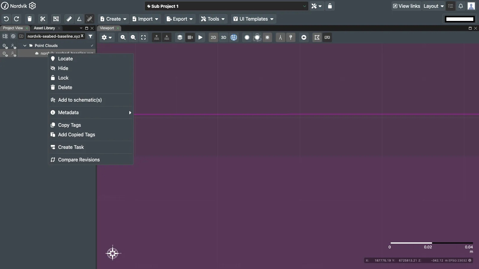
The top of the panel is where you choose what to compare. There are two slots:
A - the earlier survey, your reference.
B - the later survey, the one you are checking.
 Each slot has two dropdowns: the point cloud on top, the survey (revision) underneath.
Slot A - pick the point cloud in the first dropdown, then the survey date in the second.
Slot B - do the same. Leave the same point cloud selected to compare two of its revisions, or choose a different point cloud to compare two separate surveys.
 The dropdown lists the point clouds you can compare. Type to filter a long list.
As soon as both slots hold two different surveys, the three tool tabs appear and both surveys start loading into the 3D view.
Comparing two different surveys?
Select two point clouds first (click one, then Ctrl/Cmd-click the other) and the menu offers Compare Point Clouds instead. That fills both slots for you.
In View Checkbox - If checked only lists point clouds that overlap what you are currently looking at. If unchecked then lists everything in the project. Turn it off if a survey you expect is missing from the list.
Crosshair Icon - Jumps the 3D view to that point cloud. Handy, when you cannot see it.
Swap A / B - Swaps the two slots.
Which survey goes in which slot matters
Everything downstream is calculated as B minus A. Put the older survey in A and the newer in B, and a positive number then means material was added. If your deposition and erosion look swapped, that is what happened - press Swap A / B.
If the dropdown lists are empty then the following might help you:
| Panel Description | What to do |
|---|---|
| No point cloud in the current view… | Untick In view, or navigate to the survey. |
| No point cloud in this project. | Nothing to compare - import a survey first. |
| No processed revision yet. | The survey is still converting, or the import failed. |
| Only one comparable revision. | That point cloud has just one survey - pick a second point cloud for the other slot. |
| Pick two different revisions to compare them. | Both slots ended up on the same survey. |
Blend Tab
The Blend tab crossfades the two surveys in place. Anything that moved appears to shift or shimmer as you drag; anything that stayed put does not move at all. Nothing is computed on the server, so it is instant.
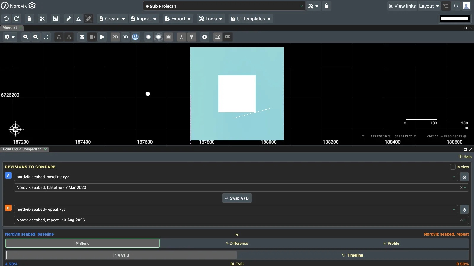 The Blend tab. The slider is at 50%, so you are seeing half of each survey.
A vs B Tab
Make sure A vs B is selected (it is by default). Drag the slider. For A a 100% value on the far left shows only the older survey. For B a 100% value on the far right shows only the newer one.
Park the slider where the change is clearest. The two dates under the slider tell you which end is which.
 Move the slider slowly around the midpoint to make local change shimmer against stable ground.
Slider - Fades survey A out while survey B fades in. The readout above shows the mix.
Clear from 3D view - Removes both surveys from the 3D view and stops the fade. Your choices in the pickers are kept.
Load now / Retry - Only appears if loading has not started or failed.
What to look for?
Drag slowly, back and forth, over a small range in the middle. Real change makes a feature jump between two positions. If the whole seabed shifts evenly, that is a datum or registration difference between the two surveys, not change on the ground.
Timeline Tab
If your point cloud has three or more surveys, Timeline steps through all of them in date order instead of just the two in the slots.
 Timeline mode. This point cloud has only one processed survey, so the tab explains that instead of showing the slider.
Revision blend slider - A continuous run across all the surveys. Stop on a whole number to see one survey; between two you get a fade of that pair.
Readout above the slider - The survey on the left, the mix percentage, the survey on the right.
Numbered list - Every survey with its date. The one or two feeding the current view are highlighted.
Timeline needs at least two processed surveys on the point cloud in slot A. If your surveys were imported as separate point clouds rather than as revisions of one, there is nothing to walk through - use A vs B and change the pair by hand.
Loading pauses while you drag
Only the surveys either side of the slider are held in memory, plus the next one along. Dragging fast across a long timeline can show a brief Loading adjacent revisions… - let go and it catches up
Difference Tab
The Difference tab turns “something moved” into a picture with numbers behind it. It works in three numbered steps that unlock in order.
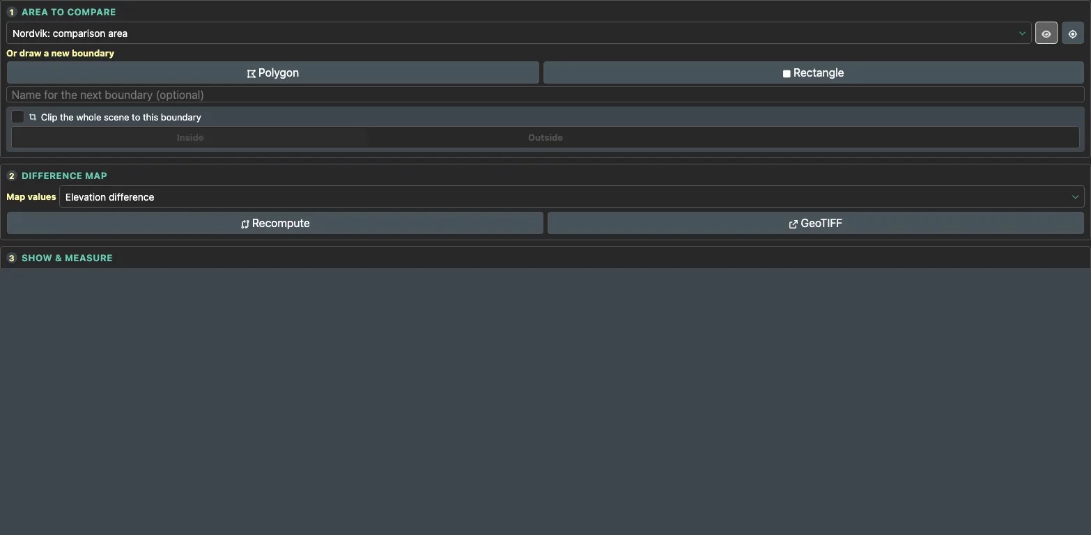 Steps 1 and 2. Step 3 appears once the map has been computed.
Area Selection
Step 1 - Choose the area
The comparison always runs inside a closed boundary. That keeps the job quick and makes the volume number mean something specific: “this much moved, in this area”.
Name for the next boundary - Type a name in if you want one - it makes the shape easy to find later. This is optional.
Polygon - In the survey in 3D view click each corner, then right-click to close the shape.
Rectangle - Click once to place it.
Press Esc to cancel, or click the same button again

The new shape becomes the selected boundary.
Once a boundary is selected, Compute difference in step 2 becomes available.
Make the area a bit bigger than the change
Include some ground that definitely did not change. It gives you a reference in the colours and in the profile, and it keeps the edge of the area away from the feature you are measuring.
Reuse an area
Pick it from the Select a boundary dropdown. Boundaries are ordinary project shapes, so they stay in the project and can be reused for every survey pair. If that area has already been compared for these two surveys, the saved result loads straight away - no waiting.
Eye - Shows or hides the selected boundary in the 3D view.
Crosshair - Jumps the 3D view to the boundary.
Cut the 3D view to the area
This is optional, but has some benefits.
Clip the whole scene to this boundary . This hides everything outside (or inside) your area in the 3D view, so you can look at the change with nothing in front of it.
Inside / Outside - Chooses which side to keep.
This only changes what you see - it never changes what is computed. It needs a simple, convex boundary without holes; with anything more complex the control is greyed out.
Compute the map
To start Step 2 then select:
Compute difference - The work happens on the server. The panel shows which step it is on and how far along it is. You can close the panel and keep working - reopening it picks the job back up.
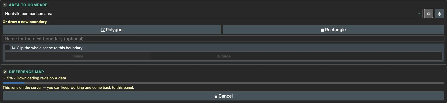 The stored job keeps running when the panel is closed and reconnects when it is opened again.
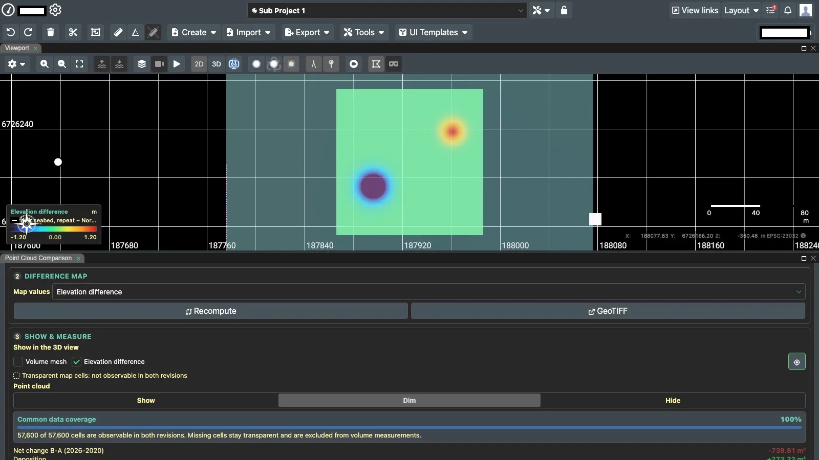
When it finishes, the change is coloured on the seabed and step 3, Show & measure, appears.

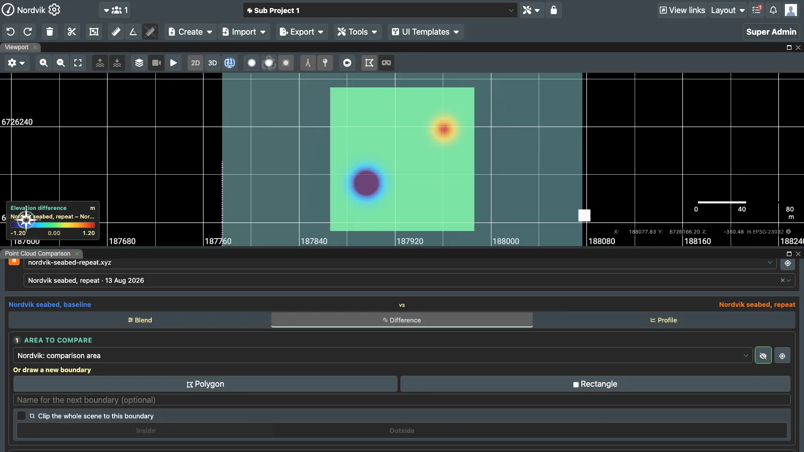 The coloured surface is the elevation change. The legend bottom-left of the 3D view gives the scale.
How long it takes depends on how big the area is and how dense the surveys are - typically a couple of minutes. Cancel discards the run.
What to show on the map
Once the map exists, Map values offers four views of the same comparison:
| Map values | Unit | Read it when |
|---|---|---|
| Elevation difference | Length | Always. This is the change itself: how much higher or lower. |
| Slope of the difference | Degrees (°) | Finding the edges of a change - the rim of a scour pit, the boundary of a backfill. |
| Ruggedness of the difference | Length | Telling rough, patchy change apart from smooth change. |
| Roughness of the difference | Length | Spotting isolated spikes, which are often data artefacts. |
Slope is the only one in degrees. The other three are lengths, so the legend carries the project’s CRS unit - m on a metric CRS, ft on one in feet.
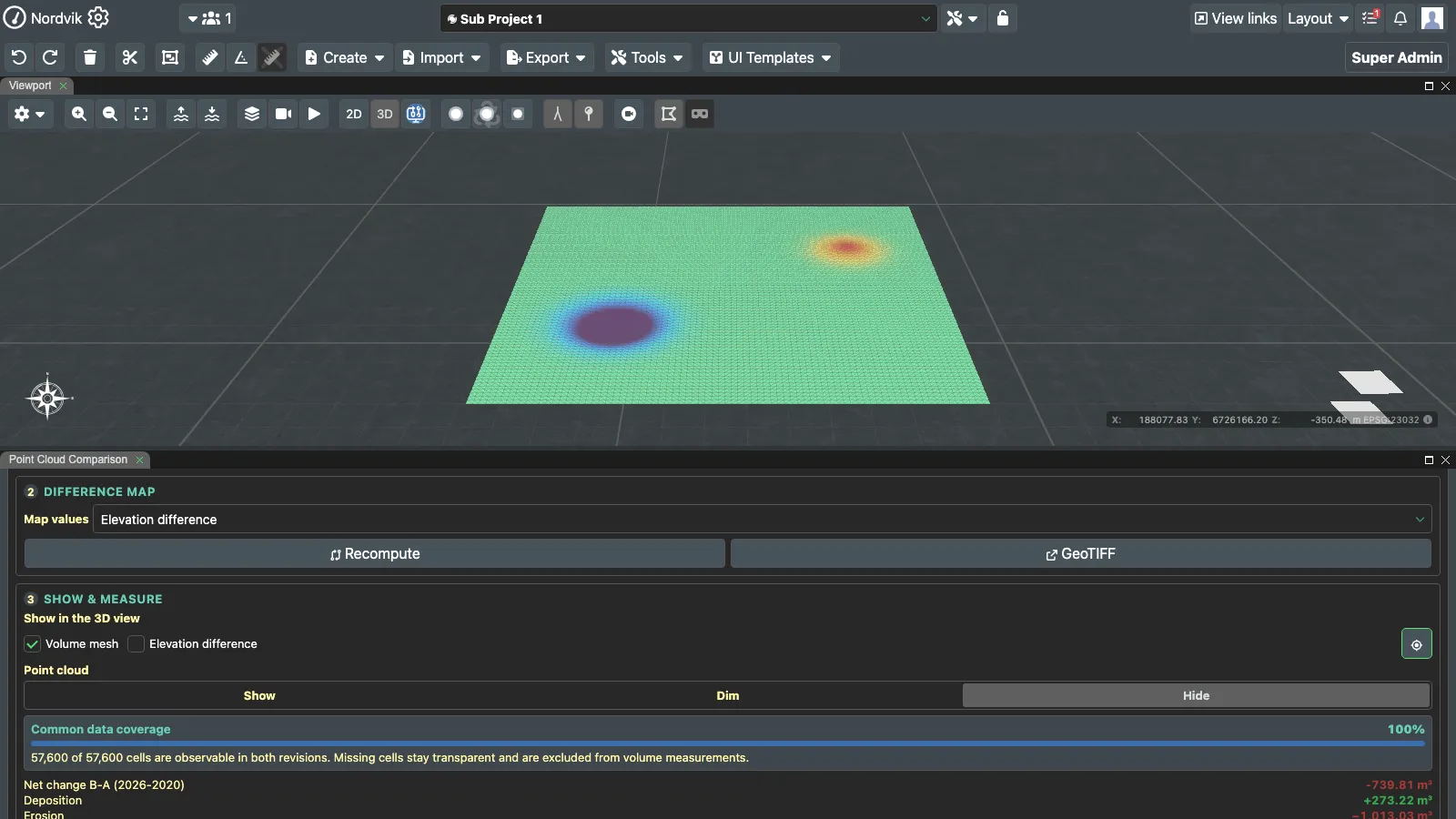 The volume mesh follows the computed cell surface inside the selected boundary.
The last three describe the change, not the seabed
“Slope of the difference” is how steeply the amount of change varies from place to place. It is not the steepness of the ground.
Recompute - Deletes this map and computes it again from the current surveys and boundary. Asks first. Use it after re-importing a survey.
GeoTIFF - Opens the map you are looking at as a GeoTIFF in a new tab, for QGIS or any other GIS.
Measure
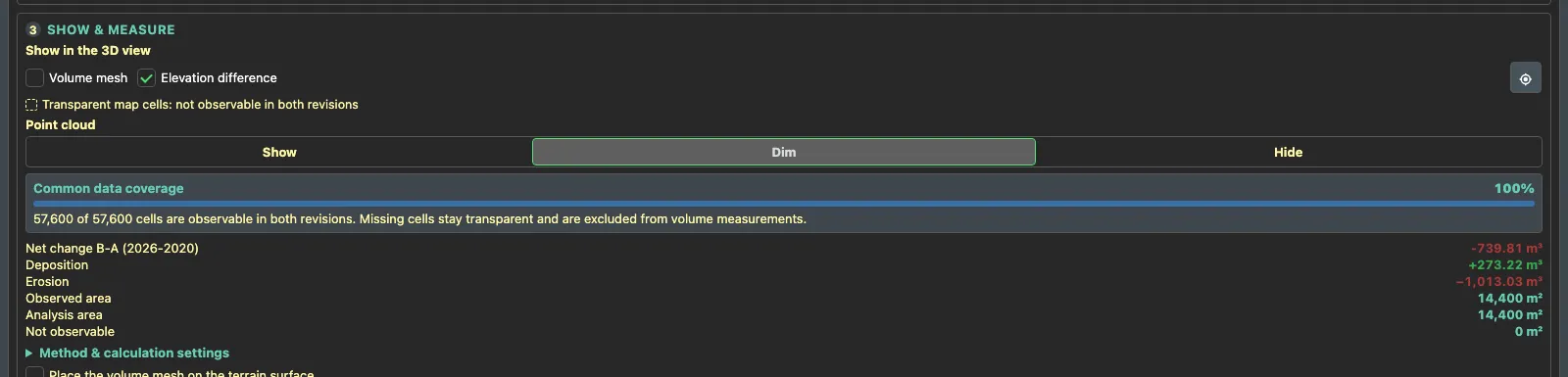
Step 3, Show & measure, appears once a difference map exists. It is where the map becomes numbers.
 A real result: 42.5% common coverage, 71 m³ net loss over a 2,142 m² area.
Read the coverage
Common data coverage is the single most important number on this panel, and it is easy to skip.
It tells you what share of your area both surveys could actually see. Where only one survey has data, there is no difference to calculate, so those cells are left out - they stay transparent on the map and contribute nothing to the volumes.
3,640 of 8,568 cells are observable in both revisions. Missing cells stay transparent and are excluded from volume measurements.
Coverage tells you what the numbers cover - not how good they are
At 42.5% coverage, the volumes below describe that 42.5% of your area. They are not an estimate for the whole area you drew. Either shrink the boundary to the part both surveys cover, or quote the coverage alongside the volume.
The measurements
You will the see the following rows of measurements. See below for what they represent:
Net change B-A - Everything added minus everything removed. Negative means the seabed is lower than before.
Deposition - Total volume gained, where the newer survey is higher.
Erosion - Total volume lost, where the newer survey is lower.
Observed area - The area both surveys covered.
Analysis area - The area of the boundary you drew.
Not observable - The difference between the two - area only one survey saw.
Areas and volumes are the project’s CRS unit squared and cubed - m² and m³ on a metric CRS, ft² and ft³ on one in feet. Nothing is converted: the figures are in the unit the coordinates are stored in. They update by themselves whenever the map or the boundary changes; Computing bounded volume… means it is working.
Where the label B-A comes from
When the two surveys are from different years the label spells it out - for example Net change B-A (2026–2020) - so nobody has to guess which way round the subtraction went.
Show it in the 3D view
Here you have two options and check the one you are interested in:
Volume mesh - The changed volume as a 3D body, coloured the same way as the map.
Elevation difference - For the map you picked. The coloured map draped on the seabed.
Crosshair button - Jumps the 3D view to whatever is currently shown.
The volume mesh is a simplified preview of the shape. The volume figures come from the full-resolution map, not from this mesh.
Place the volume mesh on the terrain surface - Drops the mesh onto the seabed instead of floating it at mid-height. Presentation only; it changes no number.
Disable Point cloud
An overlay competes with the survey points underneath it. Point cloud decides who wins:
Use the following commands to control this:
Show - Survey points at full strength.
Dim - Points faded right back, so the overlay stands out but you keep your bearings.
Hide - Overlay only.
The control is greyed out when nothing is overlaid - there would be nothing to dim for.
Change colours and range
Map colours & range is folded away because most of the time you never need it.
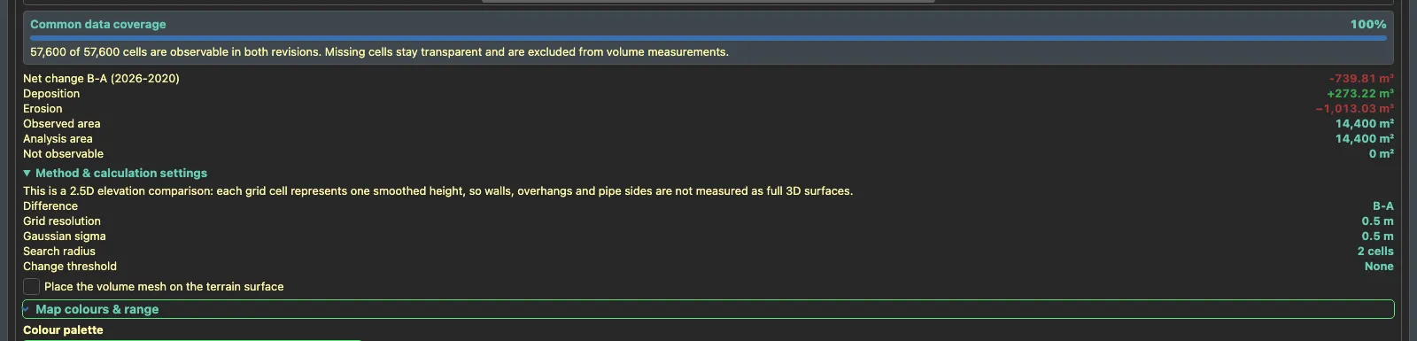 The Map colours and range section, with four palettes, layer opacity and a min and max display range
Use the following commands to control this:
Colour palette - Four colour ramps to choose from.
Layer opacity - How solid the map is drawn, 5% to 100%.
Display range - Which values the colours are spread across, as a minimum and a maximum.
Two things to expect:
-
Values outside the range take the end colour. Narrowing the range increases contrast; it never changes the data.
-
For Elevation difference the range stays symmetric around zero, so “no change” always sits in the middle of the palette. For the other three maps, which cannot be negative, it starts at zero.
Your palette, opacity and range are saved on the result, so the map looks the same for everyone the next time it is opened.
Check method and numbers
Method & calculation settings records what actually produced this result.
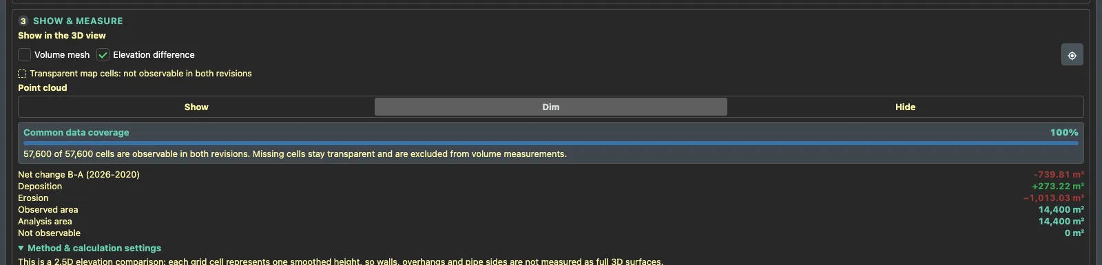 The Method and calculation settings block, showing the 2.5D caveat and the grid settings
It opens with the caveat that matters most
This is a 2.5D elevation comparison: each grid cell represents one smoothed height, so walls, overhangs and pipe sides are not measured as full 3D surfaces.
In practice that means the tool measures material moved on the seabed well, and vertical faces badly. A pipe that shifted sideways shows up as a trench beside a ridge, not as a displaced cylinder.
The settings below it - grid resolution, smoothing, search radius, change threshold - are stored with the result, so a comparison run last year is still interpretable today. How the difference is computed explains what each one does.
Compare along a line
The Profile tab draws a cross-section: distance along a line on the bottom, elevation up the side, one coloured curve per survey. It answers “how much lower is it right here” with a number you can point at, which a coloured map cannot.
It needs no boundary and no waiting - the chart appears a second or two after you draw the line.
 The Profile tab before you draw anything. Everything except Draw line waits for a line.
Draw a line
How to draw a line:
-
Optionally type a name in Name for the next line. Click
-
Draw line.
-
Click two points in the 3D view, across the feature you care about.
The chart appears:
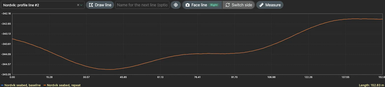 Both surveys along a 93 m line. Blue is survey A, orange is survey B.
Lines are ordinary project shapes, so you can select one in the designer afterwards and drag either end, and the chart follows.
Cross the feature, and overshoot it
Draw across the change, not along it, and extend the line into ground that definitely did not change. Where the two curves sit on top of each other, the surveys agree. If they are offset there, the two surveys disagree about the datum - and every volume you read carries that offset
To reuse a line later, pick it from the dropdown. The crosshair button jumps the 3D view to it.
Read a value off the chart
Move the pointer along the chart. A crosshair follows it and a tooltip gives you the numbers:
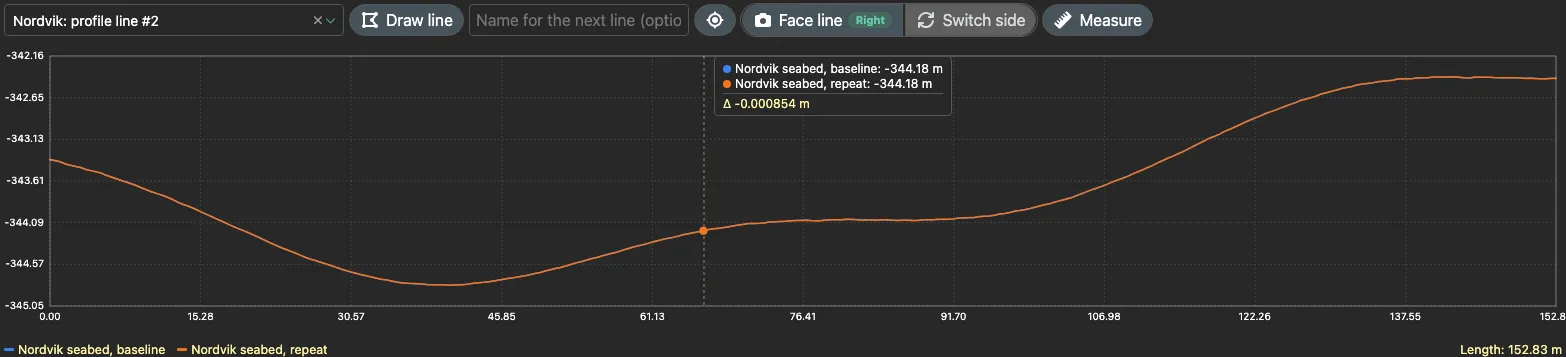 The profile chart with the cursor tooltip showing both elevations and the difference. At this station: A is −75.09 m, B is −75.23 m, so B is 0.134 m lower.
The graph elements means the following:
Blue curve - Survey A.
Orange curve - Survey B.
Δ in the tooltip - B minus A at the cursor - negative means B is lower.
Length bottom right - Total length of the line.
A gap in a curve - That survey has no data there
The chart also works from the keyboard: click it, then ← → to move the cursor (hold Shift for bigger steps), Home / End to jump to either end.
Measure between two points
To measure simply click on Measure and then click two points on the chart.
The distance and height difference between them is written on the chart.
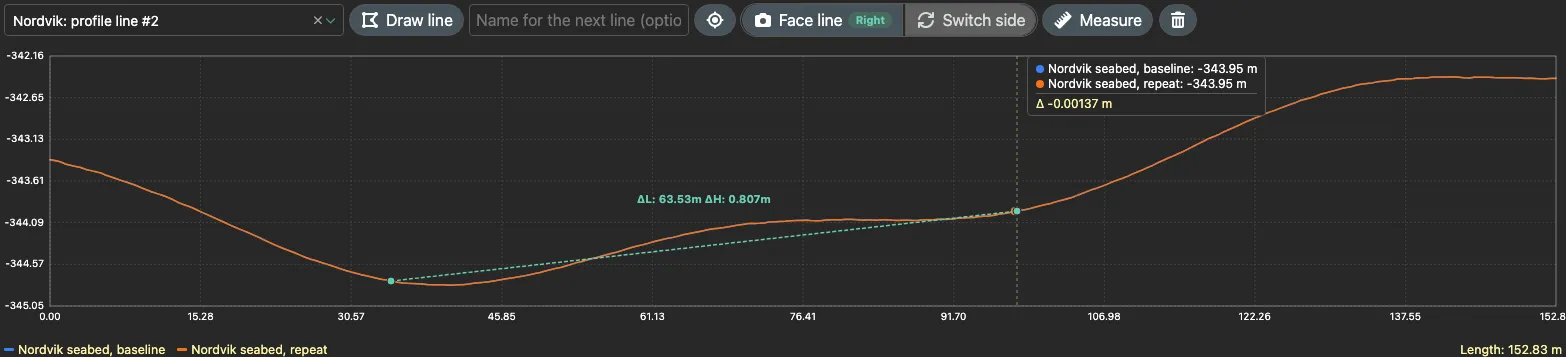 The profile chart with the cursor tooltip showing both elevations and the difference. At this station: A is −75.09 m, B is −75.23 m, so B is 0.134 m lower. And the profile chart with a measurement between two points, showing delta L 36.17 m and delta H 0.0458 m
ΔL is the horizontal distance, ΔH the height difference.
Trash button - Clears the measurement.
Enter or Space - Drops a measurement point at the cursor.
3D View on the line
This is what makes a profile convincing in a review: the 3D view showing the same cross-section as the chart.
Face line (Left / Right) - Moves the camera to look square on to the line, from the side named on the button.
Switch side - Flips both the camera and the cut to the other side.
Cut the scene along the profile line - Slices the 3D view along the line and hides everything on one side.
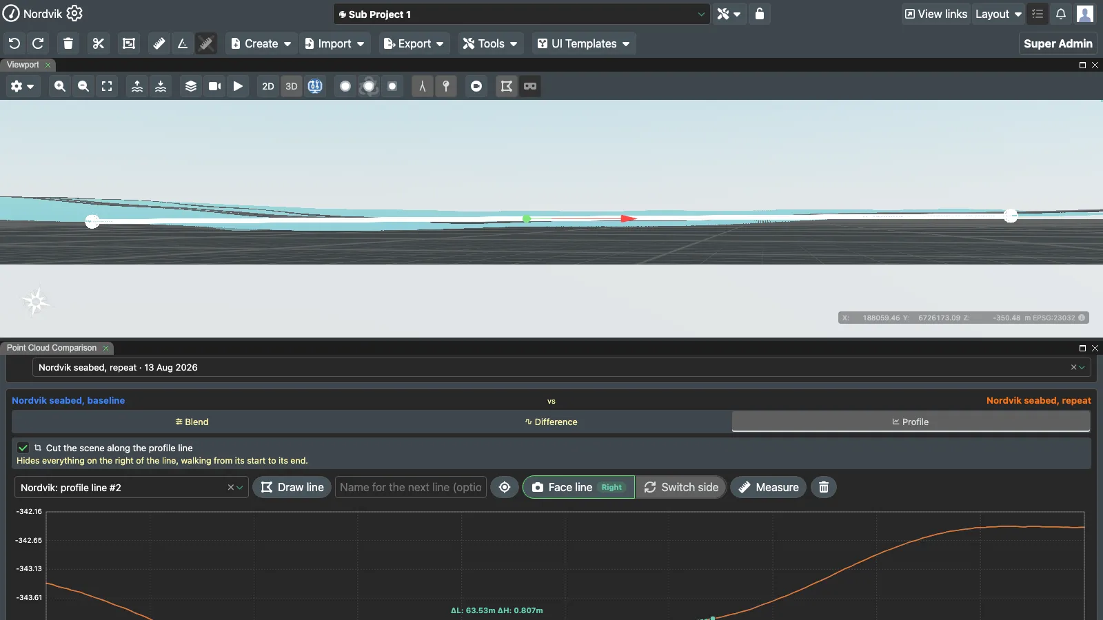 Scene cut along the line, camera facing it. The survey is now seen edge-on, matching the chart.
The hint under the checkbox names the side that will be hidden - “left” and “right” are relative to walking from the line’s first point to its last, which is why Switch side exists rather than a compass direction.
Empty Chart?
This may happen and usually that is beacuse:
| The panel says | What it means |
|---|---|
| One of the two revisions has no elevation raster yet. | One survey was imported before elevation rasters were generated. Computing a difference map for this pair fixes it as a side effect; re-importing also works. |
| No valid elevation data found along this line. | The line misses the surveys, or crosses only gaps. Redraw it over the data. |
| Select a line above, or draw a new one… | No line is selected yet. |
The chart and the map read slightly different sources
The map compares grids built from the raw survey points at the moment you press Compute difference. The chart reads each survey’s own elevation raster from when it was imported. They agree on real change, but absolute values can differ a little. Trust the map for volumes, the chart for shape and local Δ.
Every control, explained!
Use this page when you know what you are looking at but not what it does. Controls are listed in the order they appear down the panel.
Revisions to compare
This is on the top of the panel:
| Control | What it does | Greyed out when |
|---|---|---|
| In view checkbox | Limits the point cloud lists to clouds that overlap what you are looking at. | |
| Point cloud dropdown (A) | Which point cloud slot A uses. | |
| Crosshair (A) | Jumps the 3D view to point cloud A. | No point cloud picked |
| Revision dropdown (A) | Which survey of that cloud. Lists only fully processed surveys. | The cloud has no processed survey |
| Swap A / B | Swaps the two slots, flipping the sign of every result. | Nothing to swap |
| Point cloud dropdown (B), crosshair, revision dropdown | As slot A. |
The Tab row
| Control | What it does |
|---|---|
| Labels above the tabs | The two surveys being compared: A on the left in blue, B on the right in orange. |
| Blend | Fade one survey into the other in the 3D view. |
| Difference | Compute and measure a difference map. |
| Profile | Compare a cross-section along a line. |
The tab row is keyboard navigable: ← → move between tabs, Home / End jump to the first or last.
Blend tab
| Control | What it does | Greyed out when |
|---|---|---|
| A vs B | Fade between exactly the two surveys in the slots. | |
| Timeline | Walk through every processed survey of point cloud A in date order. | |
| Blend slider | 0% = only A, 100% = only B. | Surveys still loading |
| Clear from 3D view | Removes both surveys from the 3D view. Selections are kept. | |
| Load now / Retry | Starts (or retries) loading the pair. Only shown when loading has not started or has failed. | |
| Revision blend slider (Timeline) | Position across all surveys. Whole numbers show one survey; in between is a fade. | Fewer than two processed surveys |
Difference Tab - Step 1
This is for Area to compare:
| Control | What it does | Greyed out when |
|---|---|---|
| Select a boundary | Which existing shape bounds the comparison. Polygons and rectangles only. | No usable shape in the project |
| Eye | Shows or hides just the selected boundary. | No boundary selected |
| Crosshair | Jumps the 3D view to the boundary. | No boundary selected |
| Polygon | Draw a new polygon: click each corner, right-click to close. | A computation is running |
| Rectangle | Draw a new rectangle: one click places it. | A computation is running |
| Name for the next boundary | Names the next shape you draw. Optional, 80 characters. | |
| Clip the whole scene to this boundary | Hides everything outside (or inside) the boundary in the 3D view. View only. | Boundary is concave or has holes |
| Inside / Outside | Which side of the boundary to keep when clipping. | Clipping is off |
Difference Tab - Step 2
This is for Difference map:
| Control | What it does | Greyed out when |
|---|---|---|
| Compute difference | Starts the comparison on the server. | No boundary selected |
| Cancel | Discards a running computation. Asks first. | Nothing running |
| Retry | Runs a failed computation again. | Nothing failed |
| Discard | Deletes a failed result. Asks first. | Nothing failed |
| Map values | Which of the four maps to show and measure: elevation difference, slope, ruggedness, roughness. | No result yet |
| Recompute | Deletes this result and computes it again. Asks first. | No result yet |
| GeoTIFF | Opens the displayed map as a GeoTIFF in a new tab. That map does not exist on this result |
Difference Tab - Step 3
This is for Show & measure:
| Control | What it does | Greyed out when |
|---|---|---|
| Volume mesh | Shows the changed volume as a 3D body. | The volume has not been computed yet |
| Elevation difference (or the current map name) | Drapes the map on the seabed. | No map available |
| Crosshair | Jumps the 3D view to whatever is shown. | Nothing is shown |
| Show / Dim / Hide | How strongly to draw the survey points under the overlay. | No overlay is shown |
| Place the volume mesh on the terrain surface | Sits the mesh on the seabed instead of floating it. | No volume mesh |
| Method & calculation settings | Expands the record of how this result was produced. | |
| Map colours & range | Expands palette, opacity and display range. | |
| Colour palette swatches | Which colour ramp the map uses. Saved on the result. | |
| Layer opacity | How solid the map is drawn, 5-100%. Saved on the result. | |
| Min / Max display range | Which values the colours span. Saved on the result. |
Profile tab
| Control | What it does | Greyed out when |
|---|---|---|
| Cut the scene along the profile line | Slices the 3D view along the line. | No line selected |
| Line dropdown | Which line to profile along. | No line in the project |
| Draw line | Click two points in the 3D view to create a line. | |
| Name for the next line | Names the next line you draw. Optional, 80 characters. | |
| Crosshair | Jumps the 3D view to the line. | No line selected |
| Face line (Left / Right) | Points the camera square on to the line from that side. | No line, or no data along it |
| Switch side | Flips the camera and the cut to the other side. | No line, or no data along it |
| Measure | Then click two points on the chart to get ΔL and ΔH. | Both curves are empty |
| Trash | Clears the measurement. | No measurement |
Keyboard shortcuts
| Where | Key | Effect |
|---|---|---|
| Tab row | ← → Home End | Move between tabs |
| Profile chart | ← → | Move the cursor along the line |
| Profile chart | Shift + ← → | Move ten times as far |
| Profile chart | Home / End | Jump to the start or end |
| Profile chart | Enter / Space | Drop a measurement point (while measuring) |
| Drawing a shape | Esc | Cancel |
| Drawing a polygon | Right-click | Close the shape |
Three buttons ask before they act
Cancel, Discard and Recompute all show a confirmation first, because each of them throws away a result that took minutes to produce.